Understanding Neo4j GDS Link Predictions (with Demonstration)

Introduction

The Neo4j GDS Machine Learning pipelines are a convenient way to execute complex machine learning workflows directly in the Neo4j infrastructure. Therefore, they can save a lot of effort for managing external infrastructure or dependencies. In this post we will explore a common Graph Machine Learning task: Link Predictions. We will use a popular data set (The Citation Network) to prepare the input data and configure a pipeline step-by-step. I will elaborate on the main concepts and pitfalls of working with such a pipeline, so that we understand what is happening under the hood. Finally, I'll give some thoughts on current limitations.

Motivation

Link prediction is a common task in the graph context. It is used to predict missing links in the data - either to enrich the data (recommendations) or to compensate missing data.

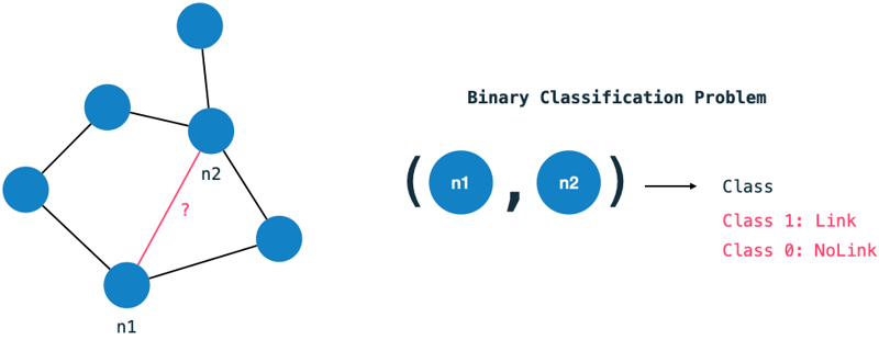
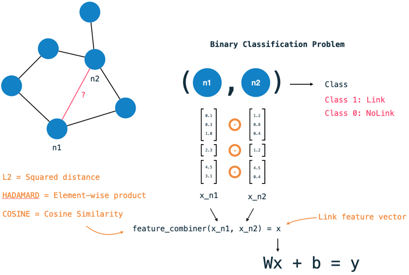
The link prediction problem can be interpreted as a binary classification problem: For each pair of nodes in the graph we ask: Should there exist a relationship between them or not? This problem statement is indeed quite verbose - we need to classify each node in the graph with each other.

The domain

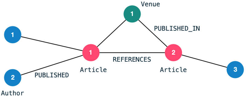
For the demonstration I will use a very commonly used data set for link prediction: The Citation Network Dataset. The dataset is publicly available can be found here. I have filtered the data to contain only a handful of publications and loaded it into a Neo4j graph. The resulting graph schema looks as follows:

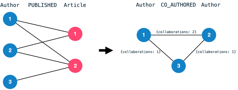
Furthermore, I have transformed the data into a homogeneous co-author graph. A co-authorship edge between two authors indicates that they have collaborated on a publication previously. The number of collaborations becomes an edge property. We transform the bipartite graph consisting of authors and articles into a homogeneous graph consisting of nodes Author and edges CO_AUTHORED.

We will work with the co-authorship graph to predict whether two authors are likely to collaborate in the future given their previous collaborations. In other words: We want to predict new CO_AUTHORED-edges.

General pipeline overview

We will use a Neo4j GDS Link Prediction Pipeline to accomplish this task (and, more importantly, to understand how to use them 😇). Let's walk through the required steps of the pipeline. You can find the official documentation here.

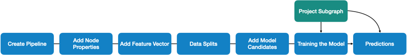
Projecting a subgraph The first step is to create an in-memory subgraph from our general graph. We use the projected graph only in the final steps of the pipeline, however, it may be easier to understand if we create it first. A projection can be created by filtering node labels and relationship types or even by custom Cypher queries. One important note for working with link prediction pipelines is that they work on undirected edges only. Therefore, we need to project our directed edges to undirected ones.

Creating the pipeline Creating the pipeline is pretty straight forward. We only need to provide a name to refer to.

Add node properties One of the most essential steps for the quality of the predictions is to use expressive features which allow the model to make the right decisions. The add-node-property step allows executing GDS graph algorithms (e.g. node embeddings) within the pipeline to generate new node features. The limitation for the algorithms (currently) is that they need to generate features for the nodes - as opposed to edges (we will discuss this later).

Add link features The feature vector step is one of the major differences to traditional ML tasks. Rather than classifying a single datapoint, we want to classify a pair of nodes. To generate a link feature vector for each pair of nodes, we use the feature vectors of both nodes and combine them into a single vector. The link-feature-vector step defines how to generate a link vector for a node pair from the individual node features. First, we need to specify which node features to use. Secondly, we have the choice of three combiner functions:

• Hadamard = Element-wise product,
• Cosine = Cosine Similarity (angle between vectors),
• L2 = Squared Distance.

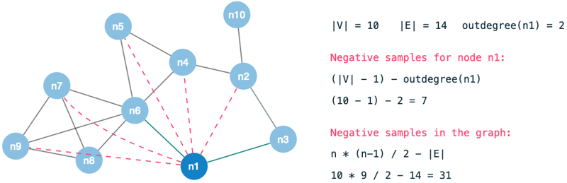
Data splitting ... looks like a trivial point in this pipeline. However, it is an essential part to understand whether you final model is useful or not. As we are classifying pairs of nodes rather than individual nodes, we end up with many combinations (|V| - 1) for each data point in the graph. Unless we are dealing with a close to fully-connected graph, there are naturally many combinations (|V| - 1 - degree(n)) without an edge for each node. These would end up being negative samples to our model and therefore a model which predicts NO-EDGE would yield high accuracy.

To circumvent this, we do the following:

• Take all existing edges which constitute the positive samples in the graph (POS)
• Split the positive samples into three distinct sets (POS = POS_TEST + POS_TRAIN + POS_FEATURE)
• For each of the three sets, sample negative examples from the graph (e.g. TEST = POS_TEST + NEG_TEST).

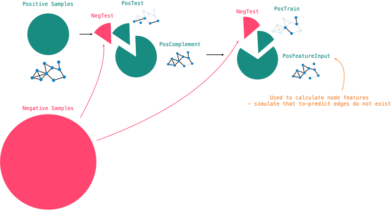
The FEATURE set is used to calculate the node features configured earlier. This is an important distinction and prevents data leakage into the train and test sets. We will discuss this a little in the Common Pitfalls section.

Notes on negative sampling: Usually we want to find one negative sample for each positive. The approach to finding good negative samples is a research topic in itself, and many approaches exist. The Neo4j GDS only supports random sampling.

Model configuration & training Currently, there exist two classification approaches in the Neo4j GDS: Logistic Regression and Random Forests. We can add multiple model candidates with various parameter spaces to the pipeline. During training, each model candidate is subject to a k-fold cross validation to find the best model configuration. Another important parameter for the training is the evaluation metric to use. The GDS offers one metric for Logistic Regression so far: AUCPR (area under curve precision-recall). The winning model is stored under the provided model identifier for later usage.

Prediction The prediction step applies the winning model to predict missing edges between all pairs of node in the graph, which do not have an edge. As this leads to a very large number of node pairs to evaluate the model for, the process can take up quite a long time. As usual, we have the choice how to consume the results: Stream or mutate. The mutate option will create the predicted relationships in the graph projection.

Common pitfalls

The most common pitfall which produces biased results, is to leak test data into the model training. This is not so much of an issue for traditional machine learning tasks as the data points have directly associated features. However, in a graph context, we often want to generate features which take into account connections in the graph. Therefore, these algorithms analyze the surroundings of nodes. In other words: The algorithms explore relationships and other data points to determine the role, connectedness, significance or embedding of a node in the larger context. The generated features then capture this knowledge about the network structure of data.

When training a model to decide whether an edge should exist between two data points, we want to hide some data from the training step, so that we can test the model performance reliably. The model should be trained without knowing the test edges. Rather, we want to obtain a model which is capable of making a good decision based on features which are independent of such an edge. Therefore, we need to pay additional attention when generating our features: No training or test data should go into the feature generation step.

The approach to enforce encapsulation and prevent data leakage is to split the input data into the three aforementioned sets: Train, test, feature. We use the feature set to calculate node properties used in the pipeline. As the three sets are distinct, we can be certain none of the edges used for training or evaluation have influenced our feature generation.

However, at this time, the only way to accomplish this strict encapsulation is by generating the features only within the pipeline. Feature generation outside the pipeline has no information about the data splits and is therefore likely to capture graph structures which the model is trying to predict.

The implementation

Considerations

The GDS pipeline encapsulates a lot of complexity in a handful lines of code. It makes large efforts to automate such workflows and prevent the engineer from tapping into one of the many pitfalls along the way. It remains indispensable to understand the concepts and error sources in link prediction to obtain useful results.

The strong encapsulation imply reduced flexibility and customization. The following szenario is not possible with the automated workflows at the moment:

It is not possible to add a node-pair feature to the feature vector. Only node properties.

Let's consider the following example for a moment: We want to make predictions for a pair of authors (a1, a2). In addition to consider the node properties of a1 and a2, which we would combine into a single vector, we would like to consider features on the pair itself. For example, it might be valuable information to the model whether the two authors (a1, a2) have cited the same paper before.

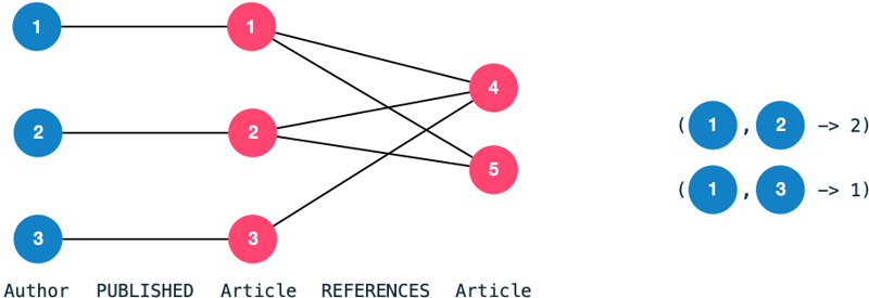
This would be a feature on the author pair, rather than on each author individually; Each author has a multiple values - one for each other author. Obviously, this feature would best be represented as an edge in the graph; It is a pair feature. In turn, if we added this feature to our pair feature vector, we wouldn't need to use a combiner as with the node features.

The major challenge with this is obviously that we needed to calculate such a feature on the various data splits to prevent data leakage. Therefore, the feature calculation either needs to happen within the pipeline (where the data splits are accessible). Or we needed to have access to the splits used for feature training, train and test.

This leads us to the second limitation with the pipelines currently:

It is not possible to configure custom splits (feature, train, test).

The pipeline allows configuration of ratios of positive samples and samples negative samples randomly. However, we cannot split our data by a custom logic - for example a timestamp. We may want data before a certain timestamp end up in the train set, whereas data after that timestamp should go to the test set. In order to accomplish this, we would need to mark our data accordingly and tell the pipeline how to use the markers in its flow. As discussed above, this custom splitting would be necessary to prevent data leakage in custom features as well.

Conclusion

The GDS Link Prediction Pipelines are a wonderful tool for setting up complex machine learning workflows directly in the Neo4j infrastructure. It reduces overhead required for external tools and resources by enabling workflows within the framework boundaries. The pipelines are simple to use and prevent many pitfalls which would require quite some thought otherwise. The API, currently, has its limitations with regard to flexibility over a custom-built solution. However, it is currently in beta version, and the GDS team may improve it in future releases.