HashGNN: Deep-dive into Neo4j GDS's new node embedding algorithm

If you prefer watching a video on this, you can do so here.

Introduction

HashGNN (#GNN) is a node embedding technique, which employs concepts of Message Passing Neural Networks (MPNN) to capture high-order proximity and node properties. It significantly speeds-up calculation in comparison to traditional Neural Networks by utilizing an approximation technique called MinHashing. Therefore, it is a hash-based approach and introduces a trade-off between efficiency and accuracy. In this article, we will understand what all of that means and will explore along a small example how the algorithms works.

Node Embeddings: Nodes with similar contexts should be close in the embedding space

Many graph machine learning use-cases like link prediction and node classification require the calculation of similarities of nodes. In a graph context, these similarities are most expressive, when they capture (i) the neighborhood (i.e. the graph structure) and (ii) the properties of the node to be embedded. Node embedding algorithms project nodes into a low-dimensional embedding space - i.e. they assign each node a numerical vector. These vectors - the embeddings - can be used for further numerical predictive analysis (e.g. machine learning algorithms). Embedding algorithms optimize for the metric: Nodes with a similar graph context (neighborhood) and/or properties should be mapped close in the embedding space. Graph embedding algorithms usually employ two fundamental steps: (i) Define a mechanism to sample the context of nodes (Random walk in node2vec, k-fold transition matrix in FastRP), and (ii) subsequently reduce the dimensionality while preserving pairwise distances (SGD in node2vec, random projections in FastRP).

HashGNN: Circumvent training a Neural Network

The clue about HashGNN is that it does not require us to train a Neural Network based on a loss function, as we would have to in a traditional Message Passing Neural Network. As node embedding algorithms optimize for "similar nodes should be close in the embedding space", the evaluation of the loss involves calculating the true similarity of a node pair. This is then used as feedback to the training, how accurate the predictions are and to adjust the weights accordingly. Often, the cosine similarity is used as similarity measure. HashGNN circumvents the model training and actually does not employ a Neural Network altogether. Instead of training weight matrices and defining a loss function, it uses a randomized hashing scheme, which hashes node vectors to the same signature with the probability of their similarity. Meaning that we can embed nodes without the necessity of comparing nodes directly against each other (i.e. no need to calculate a cosine similarity). This hashing technique is known as MinHashing and was originally defined to approximate the similarity of two sets without comparing them. As sets are encoded as binary vectors, HashGNN requires a binary node representation. In order to understand how this can be used to embed nodes of a general graph, several techniques are required. Let's have a look.

MinHashing

First of all, let's talk about MinHashing. MinHashing is a locality-sensitive hashing technique to approximate the Jaccard similarity of two sets. The Jaccard similarity measures the overlap (intersection) of two sets by dividing the intersection size by the number of the unique elements present (union) in the two sets. It is defined on sets, which are encoded as binary vectors: Each element in the universe (the set of all elements) is assigned a unique row index. If a particular set contains an element, this is represented as value 1 in the respective row of the set's vector. The MinHashing algorithm hashes each set's binary vector independently and uses K hash functions to generate a K-dimensional signature for it. The intuitive explanation of MinHashing is to randomly select a non-zero element K times, by choosing the one with the smallest hash value. This will yield the signature vector for the input set. The interesting part is, that if we do this for two sets without comparing them, they will hash to the same signature with the probability of their Jaccard similarity (if K is large enough). In other words: The probability converges against the Jaccard similarity.

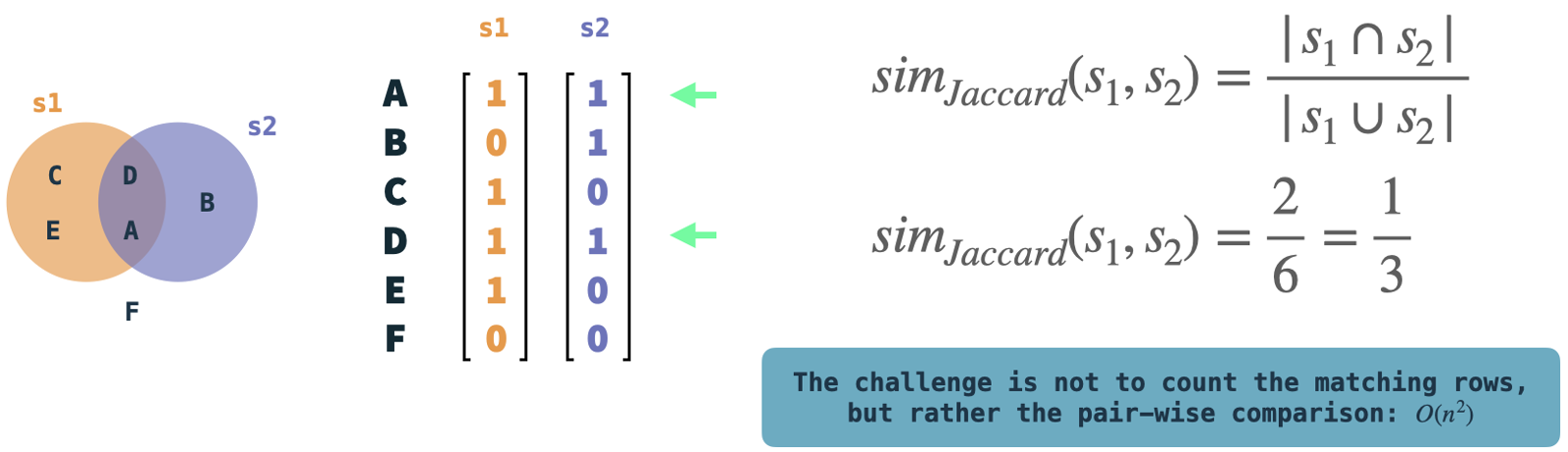
In the illustration: Example sets s1 and s2 are represented as binary vectors. We can easily compute the Jaccard similarity by comparing the two and counting the rows where both vectors have a 1. These are quite simple operations, but the complexity resides in the pair-wise comparison of vectors if we have many vectors.

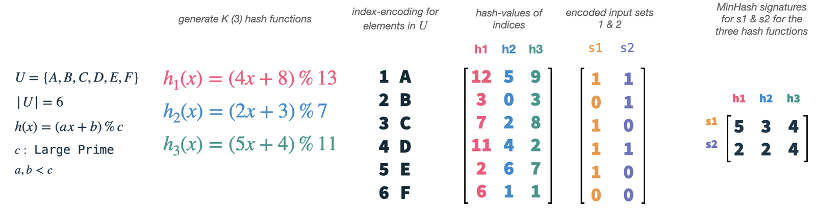
Our universe U has size 6 and we choose K (the number of hash functions) to be 3. We can easily generate new hash functions by using a simple formula and boundaries for a, b and c. Now, what we actually do is to hash the indices of our vectors (1-6), each relating to a single element in our universe, with each of our hash functions. This will give us 3 random permutations of the indices and therefore elements in our universe. Subsequently, we can take our set vectors s1 and s2 and use them as masks on our permuted features. For each permutation and set vector, we select the index of the smallest hash value, which is present in the set. This will yield two 3-dimensional vectors, one for each set, which is called the MinHash signature of the set.

MinHashing simply selects random features from the input sets, and we need the hash functions only as a means to reproduce this randomness equally on all input sets. We have to use the same set of hash functions on all vectors, so that the signature values of two input sets collide if both have the selected element present. The signature values will collide with the probability of the sets' Jaccard similarities.

WLKNN

HashGNN uses a message passing scheme as defined in Weisfeiler-Lehman Kernel Neural Networks (WLKNN) to capture high-order graph structure and node properties. It defines the context sampling strategy as mentioned earlier for HashGNN. The WLK runs in T iterations. In each iteration, it generates a new node vector for each node by combining the node's current vector with the vectors of all directly connected neighbors. Therefore, it is considered to pass messages (node vectors) along the edges to neighboring nodes.

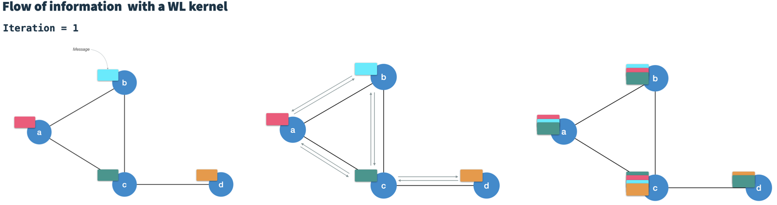
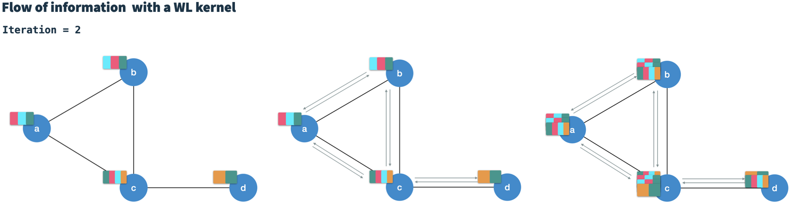
After T iterations, each node contains information of nodes at T hops distance (high-order). The calculation of the new node vector in iteration t essentially aggregates all neighbor messages (from iteration t-1) into a single neighbor message and then combines it with the node vector of the previous iteration. Additionally, the WLKNN employs three neural networks (weight matrices and activation function); (i) for the aggregated neighbor vector, (ii) for the node vector and (iii) for the combination of the two. It is a notable feature of the WLK that the calculation in iteration t is only dependent on the result of iteration t-1. Therefore, it can be considered a Markov chain.

HashGNN by example

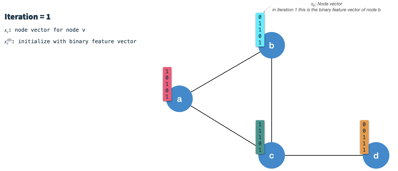
Let's explore how HashGNN combines the two approaches to embed graph vectors efficiently to embedding vectors. Just like the WLKNN, the HashGNN algorithm runs in T iterations, calculating a new node vector for every node by aggregating the neighbor vectors and its own node vector from the previous iteration. However, instead of training three weight matrices, it uses three hashing schemes for locality-sensitive hashing. Each of the hashing schemes consists of K randomly constructed hashing functions to draw K random features from a binary vector.

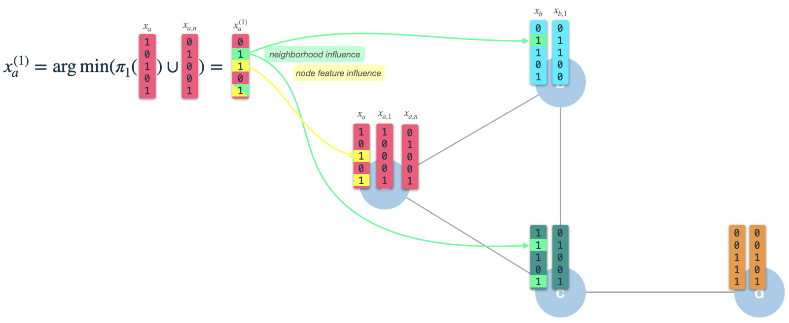
In each iteration we perform the following steps:

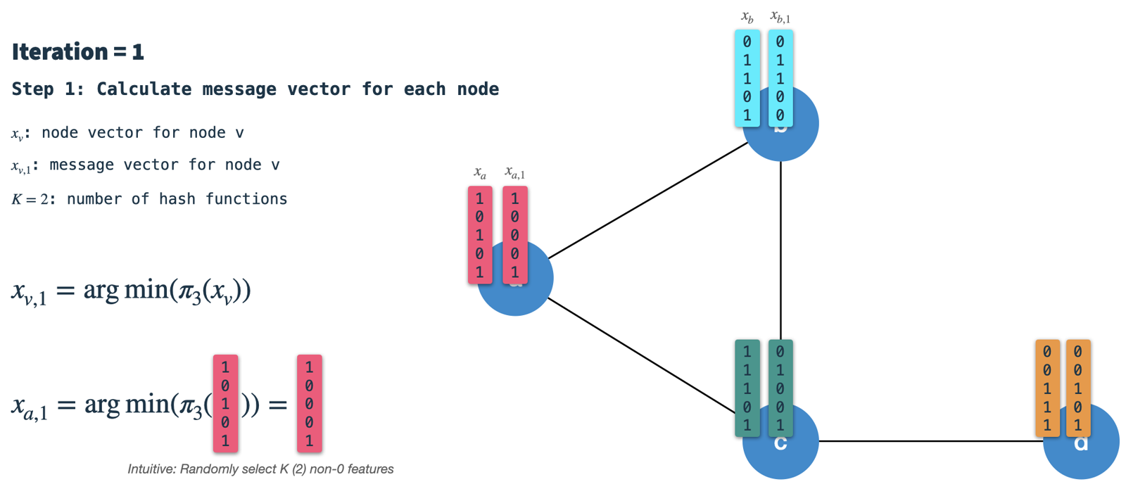
1. Calculate the node's signature vector: Min-hash (randomly select K features) the node vector from the previous iteration using hashing scheme 3. In the first iteration the nodes are initialized with their binary feature vectors (we'll talk about how to binarize nodes later). The resulting signature (or message) vector is the one which is passed along the edges to all neighbors. Therefore, we have to do this for all nodes first in every iteration.

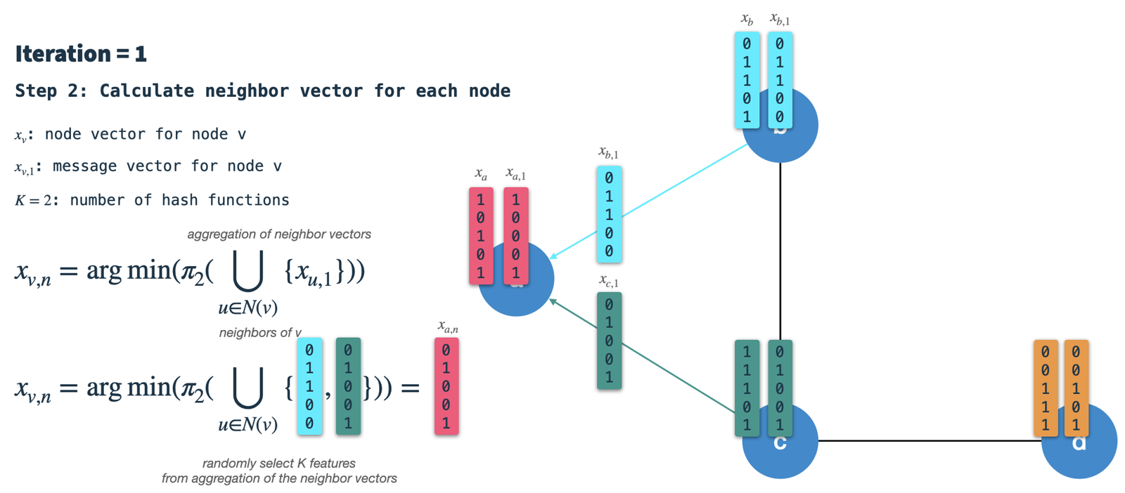
2. Construct the neighbor vector: In each node, we'll receive the signature vectors from all directly connected neighbors and aggregate them into a single binary vector. Subsequently, we use hashing scheme 2 to select K random features from the aggregated neighbor vector and call the result the neighbor vector.

3. Combine node and neighbor vector into new node vector: Finally, we use hashing scheme 1 to randomly select K features from the node vector of the previous iteration and combine the result with the neighbor vector. The resulting vector is the new node vector which is the starting point for the next iteration. Note, that this is not the same as in step 1: There, we apply hashing scheme 3 on the node vector to construct the message/signature vector.

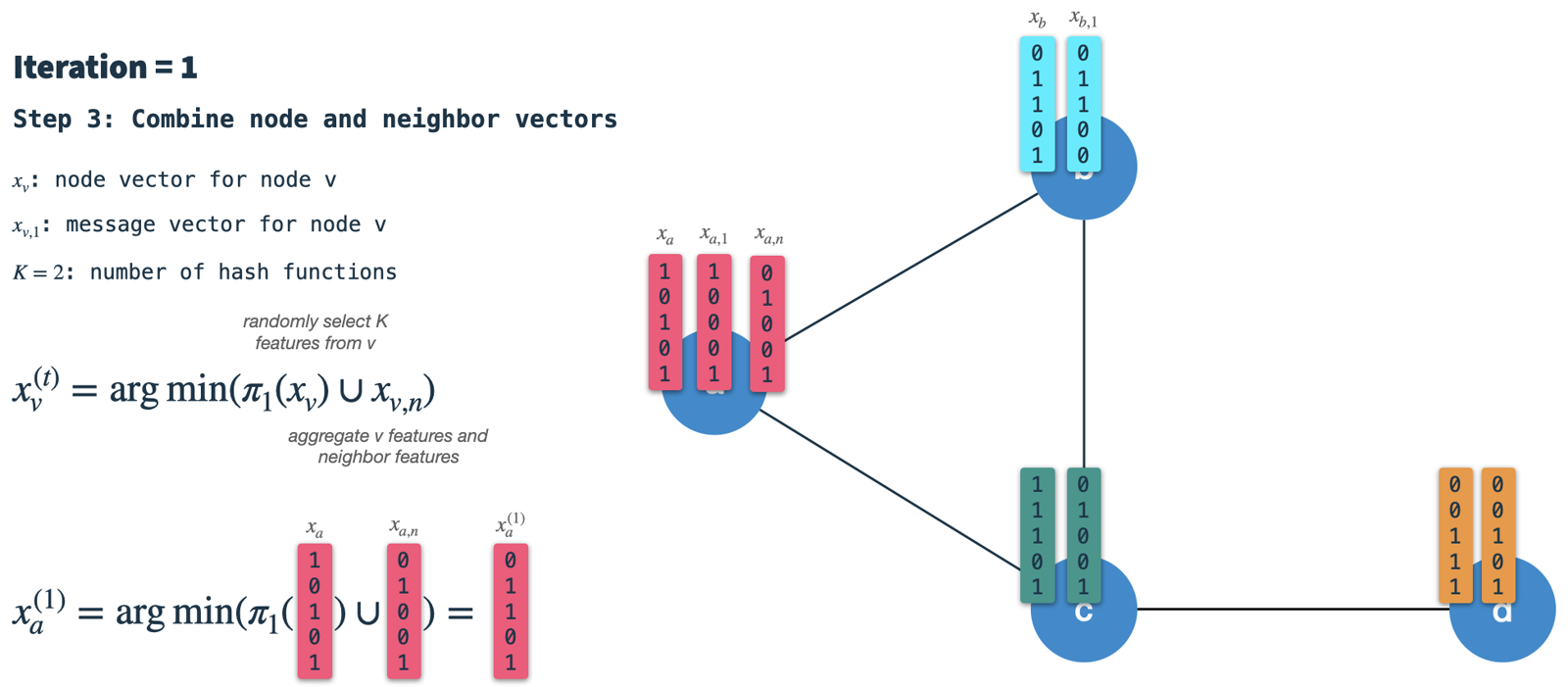
As we can see, the resulting (new) node vector has influence of its own node features (3 & 5), as well as its neighbors' features (2 & 5). After iteration 1 the node vector will capture information from neighbors with 1 hop distance. However, as we use this as input for iteration 2, it will already be influenced by features 2 hops away.

Neo4j GDS generalizations

HashGNN was implemented by the Neo4j GDS (Graph Data Science Library) and adds some useful generalizations to the algorithm.

One important auxiliary step in the GDS is feature binarization. MinHashing and therefore HashGNN requires binary vectors as input. Neo4j offers an additional preparation step to transform real-valued node vectors into binary feature vectors. They utilize a technique called hyperplane rounding. The algorithm works as follows:

1. Define node features: Define the (real-valued) node properties to be used as node features. This is done using the parameter featureProperties. We will call this the node input vector f.
2. Construct random binary classifiers: Define one hyperplane for each target dimension. The number of resulting dimensions is controlled by the parameter dimensions. A hyperplane is a high-dimensional plane and, as long as it resides in the origin, can be described solely by its normal vector n. The n vector is orthogonal to the plane's surface and therefore describes its orientation. In our case the n vector needs to be of the same dimensionality as the node input vectors (dim(f) = dim(n)). To construct a hyperplane, we simply draw dim(f) times from a Gaussian distribution.

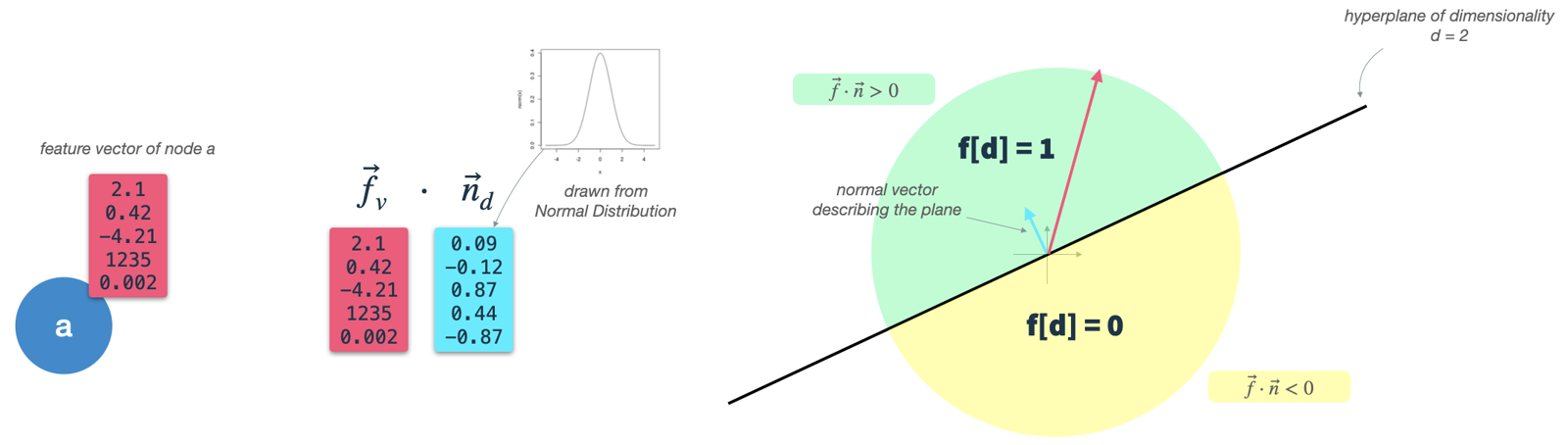
3. Classify node vectors: Calculate the dot-product of the node input vector and each hyperplane vector, which yields the angle between the hyperplane and the input vector. Using a threshold parameter, we can decide whether the input vector is above (1) or below (0) the hyperplane and assign the respective value to the resulting binary feature vector. This is exactly what also happens in a binary classification - with the only difference that we do not iteratively optimize our hyperplane, but rather use random Gaussian classifiers.

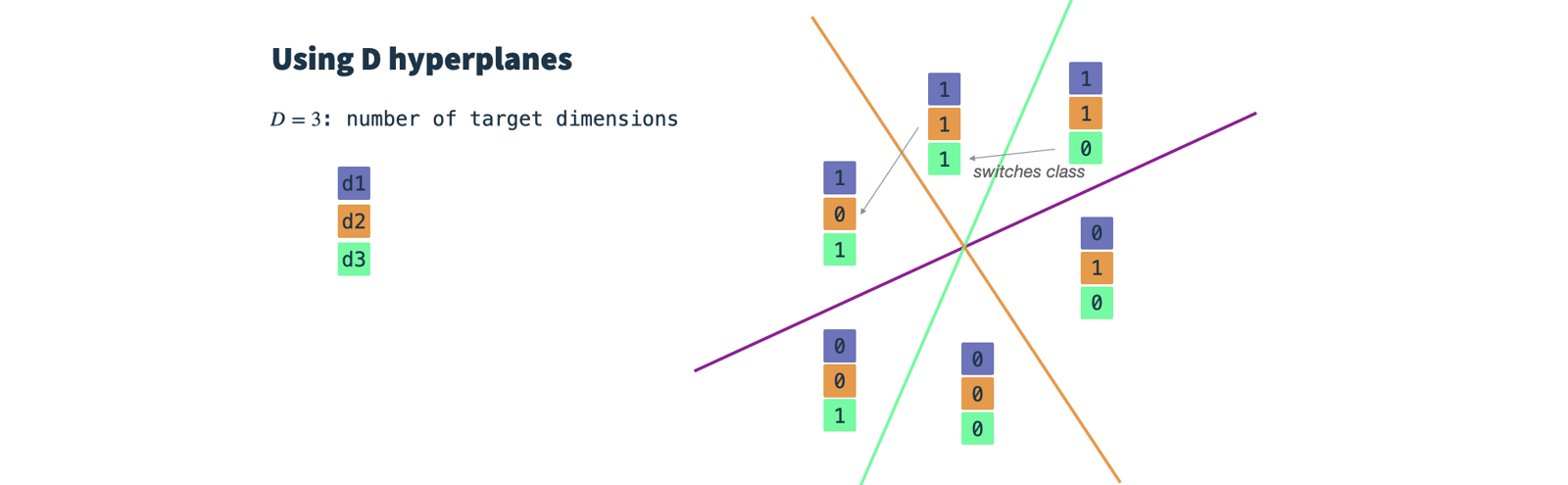
In essence, we draw one random Gaussian classifier for each target dimension and set a threshold parameter. Then, we classify our input vectors for each target dimension and obtain a d-dimensional binary vector which we use as input for HashGNN.

Conclusion

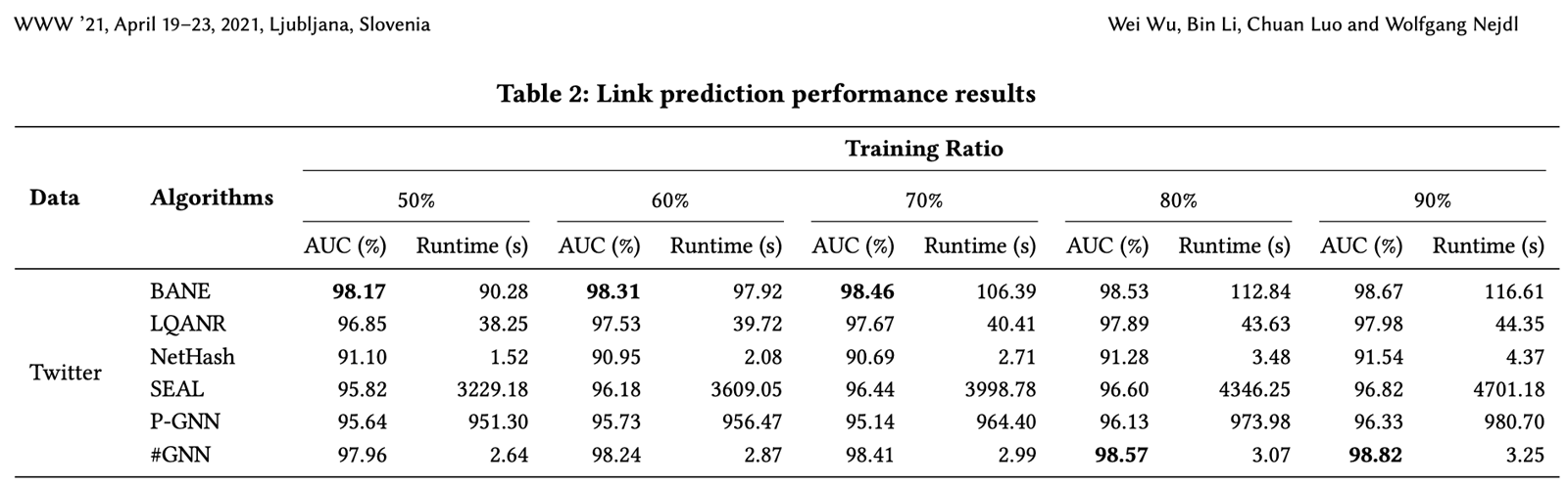
HashGNN uses locality-sensitive hashing to embed node vectors into an embedding space. By using this technique, it circumvents the computationally intensive, iterative training of a Neural Network (or other optimization), as well as direct node comparisons. The authors of the paper report a 2-4 orders of magnitude faster runtime than learning based algorithms like SEAL and P-GNN, while still producing highly comparable (in some cases even better) accuracy.

HashGNN is implemented in the Neo4j GDS (Graph Data Science Library) and can therefore be used out-of-the-box on your Neo4j graph. In the next post, I will go into practical details about how to use it, and what to keep in mind.

Thanks for stopping by and see you next time. 🚀

References

• Original Paper: Hashing-Accelerated Graph Neural Networks for Link Prediction
• Neo4j GDS Documentation: HashGNN